Some Context
Principal Components Analysis (PCA) is a tool that goes back decades used widely to identify patterns in data. Once patterns are discovered, one can compress the data by reducing the number of dimensions without much loss of information.
The objective is to transform a set of interrelated variables into a set of unrelated linear combinations of these variables. If one tries to apply PCA to a set of variables displaying low correlation, the analysis will most likely prove meaningless.
The mathematics behind PCA involves some linear algebra (primarily matrix algebra) and statistics.
Let \(E\) be a matrix containing the eigenvectors for the covariance matrix \(\hat\Sigma\) generated for our data. The eigenvectors in \(E\) become our principal components (contains the loadings). These components, by virtue of them being eigenvectors hold the following properties:
- The principal component axes are orthogonal to each other - \(e_i^Te_j = 0\) when \(i \ne j\)
- \(e_j^Te_j = 1\) \(\forall j\) (this is a condition imposed out of convenience - eigenvectors do not lose direction, therefore we can scale the length of the vectors as we wish)
From the theory of matrices, for any positive semidefinite matrix there exists an orthogonal matrix \(E\) such that:
Here, \(\Lambda\) is a diagonal matrix of non-negative values, containing the eigenvalues of \(\hat\Sigma\). If we were to consider only the first eigenvector, the first equation becomes:
Once the eigenvectors are determined, we can find the principal component scores by the following transformation:
where x is a \(N\) x \(e\) matrix, \(N\) being the number of observations and \(e\) being the number of features in the dataset. We can think of \(z\) as a rotation of the dataset \(x\) to axes defined by \(E\).
The principal component scores \(z\) are uncorrelated because
Recall \(\Lambda\) is a diagonal matrix containing the eigenvalues of \(\hat\Sigma\).
Using the eigenvalues, we can now determine which eigenvectors (components) we want to use or more importantly which ones to remove. A judgement call needs to be made with the help of the latent roots criterion and the scree test. You will inevitably lose some information by culling components but if the eigenvalues are small, you won’t lose much.
For a thorough commentary, please refer to the following link.
Workflow
The dataset I’ve used is Spotify data available on Kaggle which contains audio features for the top 100 spotify tracks at a certain period in time. The data seems fairly clean with all records containing values.
Read in the data and plot the correlation of the audio features.
data <- read_csv("featuresdf.csv",locale = readr::locale(encoding = "windows-1252"))
## Parsed with column specification:
## cols(
##   id = col_character(),
##   name = col_character(),
##   artists = col_character(),
##   danceability = col_double(),
##   energy = col_double(),
##   key = col_double(),
##   loudness = col_double(),
##   mode = col_double(),
##   speechiness = col_double(),
##   acousticness = col_double(),
##   instrumentalness = col_double(),
##   liveness = col_double(),
##   valence = col_double(),
##   tempo = col_double(),
##   duration_ms = col_double(),
##   time_signature = col_double()
## )
data_scaled <- as.data.frame(scale(data[, 4:13]))
plot_correlation(data_scaled)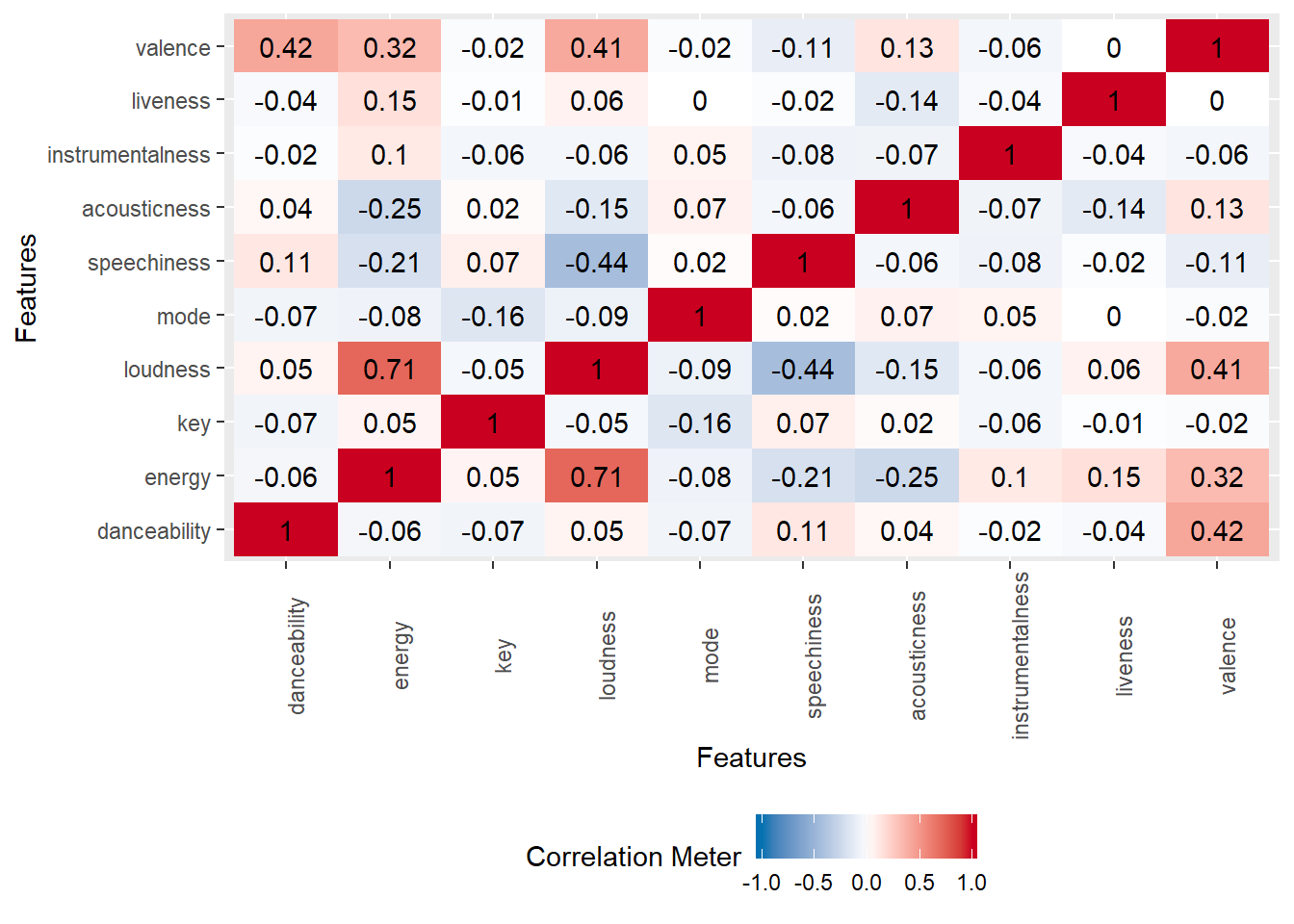
Based off the correlation matrix above, we don’t see a high correlation between the variables besides energy and loudness. This is looking bad for our PCA. Based off the above, we can suspect that we will need the majority of the components to explain the majority of the variance in the dataset. We can see this in the scree-plot below. Instead of one or two components that can explain the majority of the variance in the dataset, it looks like we need at least a half of the components.
Apply the principal() function from the psych package.
pca <- principal(data[, 4:13], rotate = "none")
plot(pca$values[1:10], type = "b", ylab = "Eigenvalues", xlab = "Component")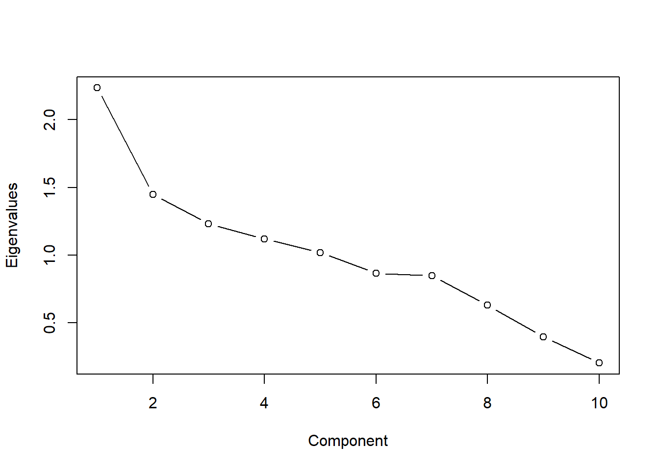
pca_5 <- principal(data_scaled, nfactors = 5, rotate = "none")
pca_5
## Principal Components Analysis
## Call: principal(r = data_scaled, nfactors = 5, rotate = "none")
## Standardized loadings (pattern matrix) based upon correlation matrix
##                    PC1   PC2   PC3   PC4   PC5   h2   u2 com
## danceability      0.16  0.75  0.11  0.39  0.17 0.79 0.21 1.8
## energy            0.83 -0.24  0.09  0.06  0.07 0.76 0.24 1.2
## key              -0.04 -0.06  0.64 -0.42  0.14 0.60 0.40 1.9
## loudness          0.91 -0.05 -0.05 -0.11 -0.06 0.84 0.16 1.1
## mode             -0.15 -0.03 -0.64  0.21 -0.29 0.56 0.44 1.8
## speechiness      -0.50  0.17  0.40  0.47  0.05 0.66 0.34 3.2
## acousticness     -0.22  0.49 -0.28 -0.55 -0.17 0.70 0.30 3.1
## instrumentalness  0.03 -0.25 -0.36  0.19  0.74 0.78 0.22 1.9
## liveness          0.17 -0.29  0.19  0.40 -0.54 0.60 0.40 3.0
## valence           0.59  0.63 -0.01  0.08 -0.02 0.75 0.25 2.0
##
##                        PC1  PC2  PC3  PC4  PC5
## SS loadings           2.23 1.45 1.23 1.12 1.02
## Proportion Var        0.22 0.14 0.12 0.11 0.10
## Cumulative Var        0.22 0.37 0.49 0.60 0.71
## Proportion Explained  0.32 0.21 0.17 0.16 0.14
## Cumulative Proportion 0.32 0.52 0.70 0.86 1.00
##
## Mean item complexity =  2.1
## Test of the hypothesis that 5 components are sufficient.
##
## The root mean square of the residuals (RMSR) is  0.11
##  with the empirical chi square  111.85  with prob <  1.7e-22
##
## Fit based upon off diagonal values = 0.62
We can see that the first component has a high loading for energy and loudness which is what we were expecting given their high correlation.
Before we investigate further, let us apply orthogonal rotation on our components using varimax. The purpose of rotating is to maximise the loadings on particular features on a specific component. This helps interpretation.
pca_rotate <- principal(data_scaled, nfactors = 5, rotate = "varimax")
pca_rotate
## Principal Components Analysis
## Call: principal(r = data_scaled, nfactors = 5, rotate = "varimax")
## Standardized loadings (pattern matrix) based upon correlation matrix
##                    RC1   RC2   RC4   RC3   RC5   h2   u2 com
## danceability     -0.13  0.88 -0.01  0.01 -0.04 0.79 0.21 1.1
## energy            0.76  0.11  0.38 -0.13 -0.06 0.76 0.24 1.6
## key              -0.03 -0.13 -0.07 -0.75  0.11 0.60 0.40 1.1
## loudness          0.89  0.19  0.13 -0.04  0.06 0.84 0.16 1.1
## mode             -0.06 -0.11 -0.08  0.73  0.03 0.56 0.44 1.1
## speechiness      -0.71  0.23  0.30 -0.12  0.06 0.66 0.34 1.7
## acousticness     -0.06  0.06 -0.81  0.08  0.19 0.70 0.30 1.2
## instrumentalness  0.04 -0.05  0.13  0.13 -0.86 0.78 0.22 1.1
## liveness          0.08 -0.08  0.57  0.18  0.49 0.60 0.40 2.3
## valence           0.41  0.74 -0.12  0.01  0.11 0.75 0.25 1.7
##
##                        RC1  RC2  RC4  RC3  RC5
## SS loadings           2.07 1.46 1.27 1.19 1.05
## Proportion Var        0.21 0.15 0.13 0.12 0.11
## Cumulative Var        0.21 0.35 0.48 0.60 0.71
## Proportion Explained  0.29 0.21 0.18 0.17 0.15
## Cumulative Proportion 0.29 0.50 0.68 0.85 1.00
##
## Mean item complexity =  1.4
## Test of the hypothesis that 5 components are sufficient.
##
## The root mean square of the residuals (RMSR) is  0.11
##  with the empirical chi square  111.85  with prob <  1.7e-22
##
## Fit based upon off diagonal values = 0.62
Now, for the first component, we can more easily determine what features are being emphasised (energy, loudness, valence and speechiness). With business domain knowledge, one can now try to categorise and define each of the components, not in terms of just one variable but by grouping variables, for e.g. energy and loudness are quite similar and can be coined as ambience for instance.
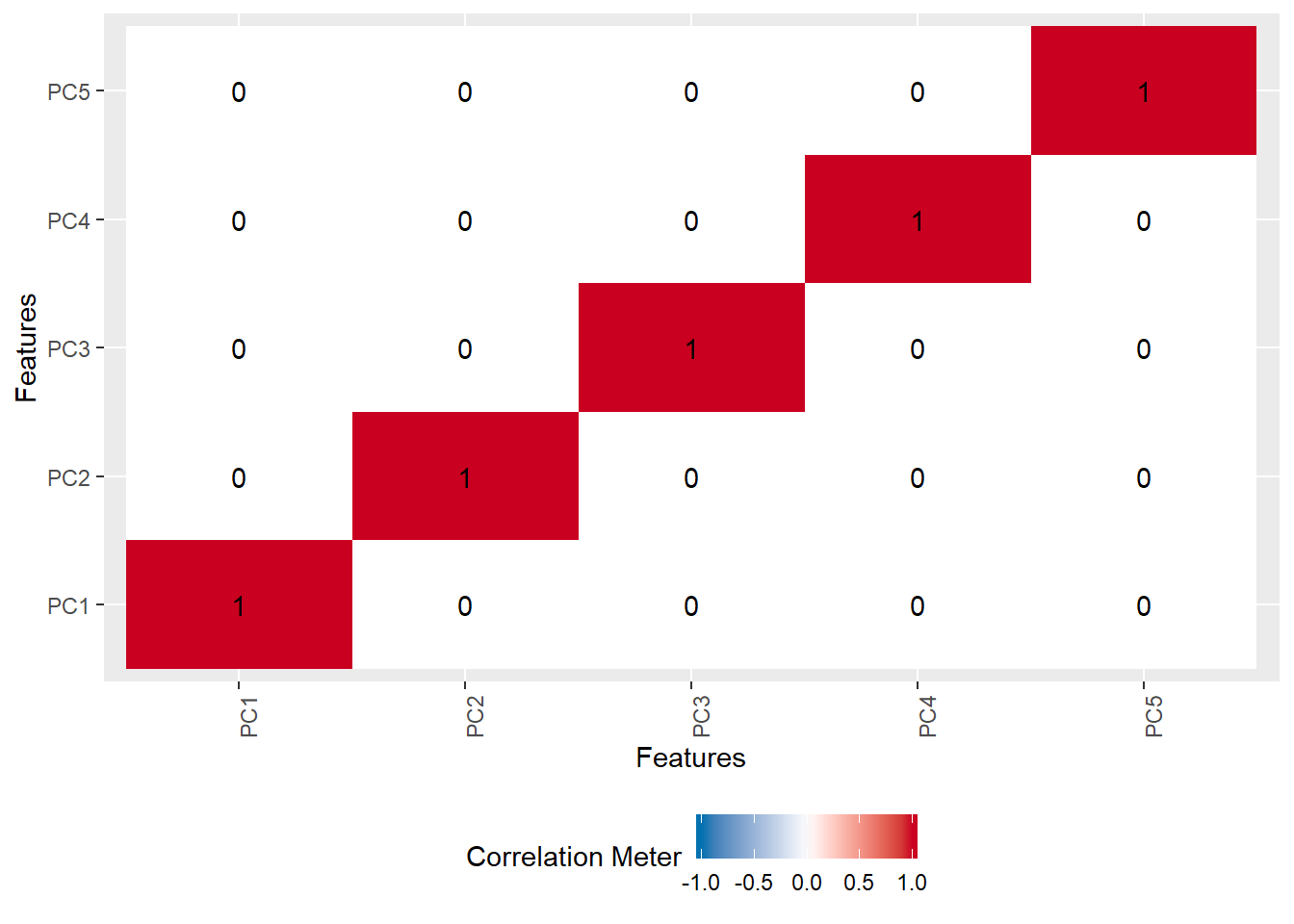
To finish off, let’s check out the correlation of our components (for both the rotated and not rotated components). They should be uncorrelated except for themselves.
pca_scores <- data.frame(round(pca_rotate$scores, digits = 2))
plot_correlation(pca_scores)
pca_5_scores <- data.frame(round(pca_5$scores, digits = 2))
plot_correlation(pca_5_scores)